Basic KLIP Subtraction Tutorial for JWST Simualted Data

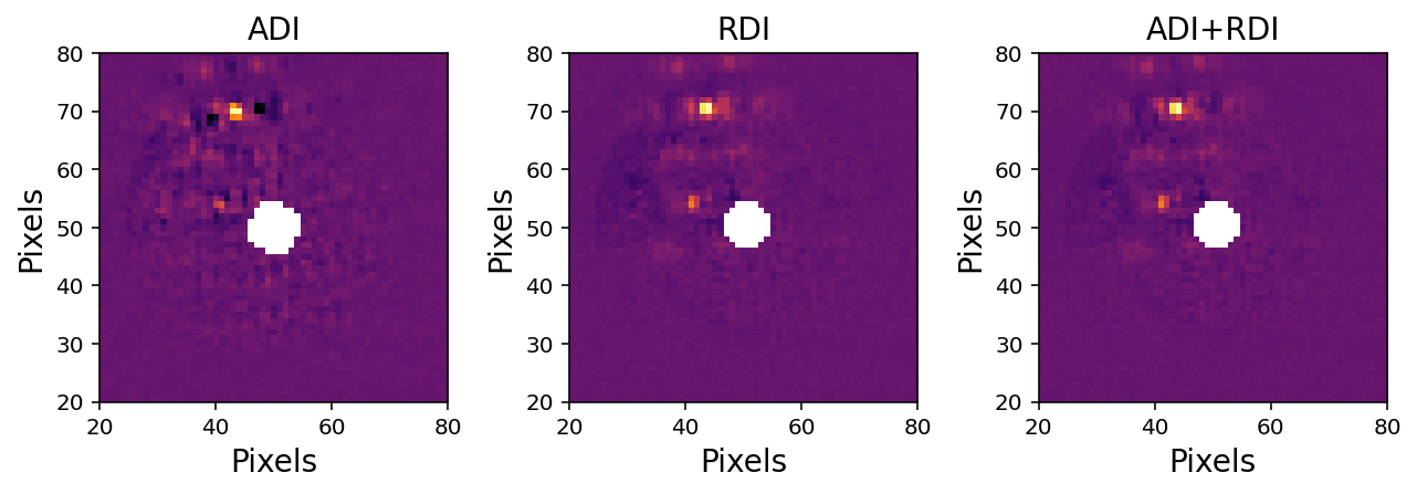
In this notebook tutorial, we’ll be demonstrating pyKLIP’s core functionality of starlight subtraction with simulated data from the James Webb Space Telescope. This data conatains two planets that we’d like to recover, and we will reduce it in three ways: Angular Differential Imaging (ADI), Reference Differential Imaging (RDI), and a combination of the two (ADI+RDI).

With ADI, we take advantage of telescope roll angles to distinguish the light from the star and the planet, and subsequently build a model of the starlight to be subtracted. These patterns are diffrentiated by the fact that we expect the planet companion to rotate between angles while the stellar PSF will stay constant.Post-subtraction, we’ll be left with the exoplanets underneath!

Alternatively, RDI makes use of another star, called a reference star to create the model of the star that we subtract. The reference star should be of a similar spectral time, but with no planets around it. We can also combine these technqiues.

NB: We’ll save the characterization of the planets we recover for separate tutorials

import os
import astropy.io.fits as fits
import numpy as np
import scipy
import scipy.ndimage as ndi
import matplotlib.pylab as plt
%matplotlib inline
%config InlineBackend.figure_format = 'retina'

import pyklip.klip
import pyklip.instruments.Instrument as Instrument
import pyklip.parallelized as parallelized
import pyklip.rdi as rdi

Read in the data

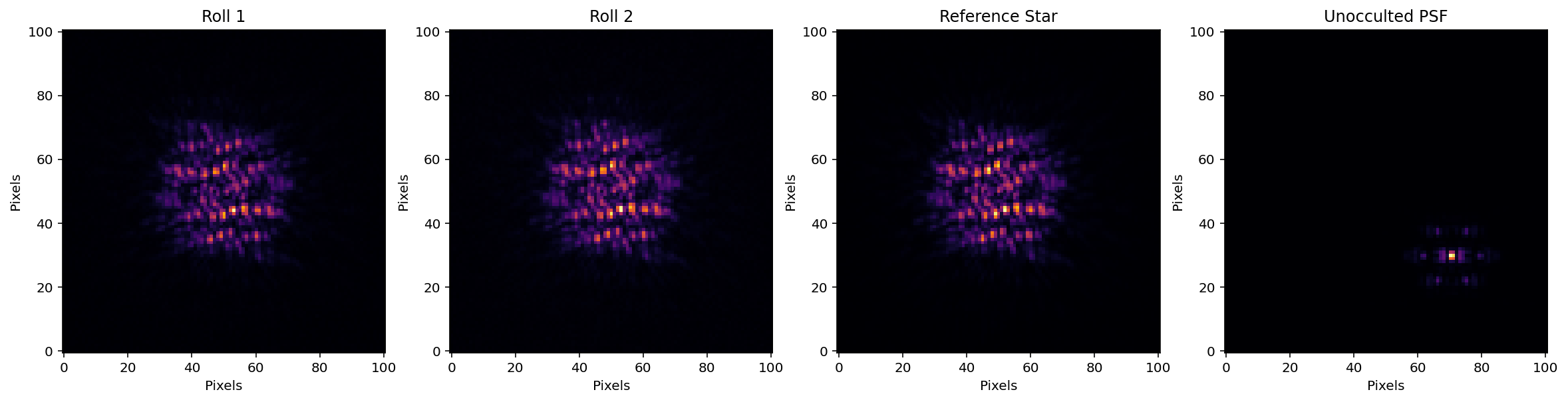
For this tutorial, we’ll use data taken of the science target at two telescope roll angles, as well as data taken on a reference star (without companions) that we can use to model the stellar PSF. Here, we don’t simulate saturation, but for real JWST, we will place the star behind an ND filter and we will know the ND throughput.

filtername = "f300m"

# read in roll 1
with fits.open("old_simulated_data/NIRCam_target_Roll1_{0}.fits".format(filtername)) as hdulist:
    roll1_cube = hdulist[0].data
    print(roll1_cube.shape)

# read in roll 2
with fits.open("old_simulated_data/NIRCam_target_Roll2_{0}.fits".format(filtername)) as hdulist:
    roll2_cube = hdulist[0].data
    print(roll2_cube.shape)

# read in ref star
with fits.open("old_simulated_data/NIRCam_refs_SGD_{0}.fits".format(filtername)) as hdulist:
    ref_cube = hdulist[0].data
    print(ref_cube.shape)

# read in unocculted PSF
with fits.open("old_simulated_data/NIRCam_unocculted_{0}.fits".format(filtername)) as hdulist:
    psf_cube = hdulist[0].data
    print(psf_cube.shape)

fig = plt.figure(figsize=(20,10))

ax1 = fig.add_subplot(1,4,1)
ax1.imshow(roll1_cube[0], interpolation="nearest", cmap="inferno")
ax1.invert_yaxis()
plt.xlabel('Pixels')
plt.ylabel('Pixels')
ax1.set_title("Roll 1")

ax2 = fig.add_subplot(1,4,2)
ax2.imshow(roll2_cube[0], interpolation="nearest", cmap="inferno")
ax2.invert_yaxis()
ax2.set_title("Roll 2")
plt.xlabel('Pixels')
plt.ylabel('Pixels')

ax3 = fig.add_subplot(1,4,3)
ax3.imshow(ref_cube[0], interpolation="nearest", cmap="inferno")
ax3.invert_yaxis()
plt.xlabel('Pixels')
plt.ylabel('Pixels')
ax3.set_title("Reference Star")

ax4 = fig.add_subplot(1,4,4)
ax4.imshow(psf_cube[0], interpolation="nearest", cmap="inferno")
ax4.invert_yaxis()
plt.xlabel('Pixels')
plt.ylabel('Pixels')
ax4.set_title("Unocculted PSF")

(6, 101, 101)
(6, 101, 101)
(54, 101, 101)
(6, 101, 101)

Text(0.5, 1.0, 'Unocculted PSF')

Read in the Data into pyKLIP

Since we’re using simulated data, we don’t yet have data with proper header information. To bypass this, we’ll use the Generic Data interface for simulated JWST data and combine the two science roll angles to produce a dataset.

# combine the two rows
full_seq = np.concatenate([roll1_cube, roll2_cube], axis=0)

# two rolls are offset 10 degrees, this is the right sign (trust me)
pas = np.append([0 for _ in range(roll1_cube.shape[0])], [10 for _ in range(roll2_cube.shape[0])])

# for each image, the (x,y) center where the star is is just the center of the image
centers = np.array([np.array(frame.shape)/2. for frame in full_seq])

# give it some names, just in case we want to refer to them
filenames = np.append(["roll1_{0}".format(i) for i in range(roll1_cube.shape[0])],
                      ["roll2_{0}".format(i) for i in range(roll1_cube.shape[0])])

# create the GenericData object. This will standardize the data for pyKLIP
dataset = Instrument.GenericData(full_seq, centers, IWA=4, parangs=pas, filenames=filenames)
dataset.flipx = False # get the right handedness of the data

Run KLIP-ADI

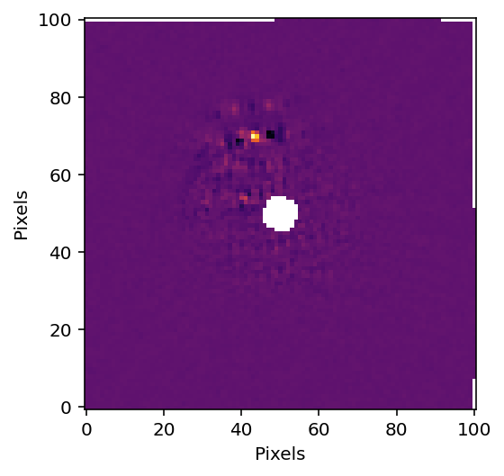
To use KLIP-ADI, we will break up the image into 9 concentric annuli and each annuli into 4 azimuthal sectors. KLIP is run on each sector independently. A free parameter of KLIP is the number of PCA (Principal Component Analysis) modes used to reconstruct the stellar PSF (the numbasis keyword). This number controls the pattern-finding in our images, and the higher it is, the more aggresive the KLIP reduction is. pyKLIP allows us to try a bunch, input as a list or array, to see which is best.

parallelized.klip_dataset(dataset, outputdir="./", fileprefix=f"pyklip-{filtername}-ADI-k50a9s4m1", annuli=9,
                          subsections=4, numbasis=[1,5,10,20,50], mode="ADI", movement=1)

Begin align and scale images for each wavelength
Wavelength 1.0 with index 0 has finished align and scale. Queuing for KLIP
Total number of tasks for KLIP processing is 36
27.78% done (9/36 completed)
55.56% done (19/36 completed)
83.33% done (29/36 completed)
Closing threadpool
Derotating Images...
Writing Images to directory /Users/jeaadams/JWST-ERS-Pipeline/notebooks
wavelength collapsing reduced data of shape (b, N, wv, y, x):(5, 12, 1, 101, 101)

# Plot this reduced data cube. The 3rd axis is the number of PCA modes used
with fits.open(f"pyklip-{filtername}-ADI-k50a9s4m1-KLmodes-all.fits") as hdulist:
    adi_cube = hdulist[0].data

plt.figure()
# plot the KL10 Cube (index of 2)
plt.imshow(adi_cube[2], interpolation='nearest', cmap='inferno')
plt.gca().invert_yaxis()
plt.xlabel('Pixels')
plt.ylabel('Pixels')

Text(0, 0.5, 'Pixels')

pyKLIP RDI Reduction

Set up PSF Library

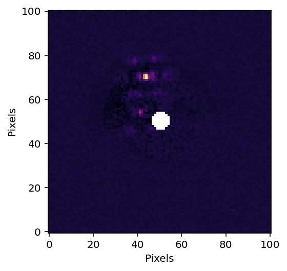
In order to use RDI, we’ll need to put all of our reference images and science images into a PSF library for pyKLIP to access. Within this PSF library, we’ll find the reference images that are the most correlated with our science images, and figure out the best stars in our library to model the stellar PSF we care about.

We assume all the simualted data is aligned to the image center

# combine both science target and reference target images into a psf library array
psflib_imgs = np.append(ref_cube, full_seq, axis=0)
ref_filenames = ["ref_{0}".format(i) for i in range(ref_cube.shape[0])]
psflib_filenames = np.append(ref_filenames, filenames, axis=0)
# all frames aligned to image center (Which are the same size)
ref_center = np.array(ref_cube[0].shape)/2

# make the PSF library
# we need to compute the correlation matrix of all images vs each other since we haven't computed it before
psflib = rdi.PSFLibrary(psflib_imgs, ref_center, psflib_filenames, compute_correlation=True)

# save the correlation matrix to disk so that we also don't need to recomptue this ever again
# In the future we can just pass in the correlation matrix into the PSFLibrary object rather than having it compute it
psflib.save_correlation("corr_matrix_{0}.fits".format(filtername), clobber=True)

pyklip.rdi.save_correlation: clobber was deprecated in Astropy version 2.0 andwill be removed in a future version. Use argument overwrite instead)

# prepare the PSF Library to run on our science dataset
psflib.prepare_library(dataset)

# Run pyKLIP RDI
parallelized.klip_dataset(dataset, outputdir="./", fileprefix=f"pyklip-{filtername}-RDI-k50a9s4", annuli=9,
                          subsections=4, numbasis=[1,5,10,20,50], mode="RDI", psf_library=psflib)

# Open and plot
with fits.open(f"pyklip-{filtername}-RDI-k50a9s4-KLmodes-all.fits") as hdulist:
    rdi_cube = hdulist[0].data

plt.figure()
# plot the KL20 Cube (index of 3)
plt.imshow(rdi_cube[3], interpolation='nearest', cmap='inferno')
plt.gca().invert_yaxis()
plt.xlabel('Pixels')
plt.ylabel('Pixels')

Begin align and scale images for each wavelength
Wavelength 1.0 with index 0 has finished align and scale. Queuing for KLIP
Total number of tasks for KLIP processing is 36
27.78% done (9/36 completed)
55.56% done (19/36 completed)
83.33% done (29/36 completed)
Closing threadpool
Derotating Images...
Writing Images to directory /Users/jeaadams/JWST-ERS-Pipeline/notebooks
wavelength collapsing reduced data of shape (b, N, wv, y, x):(5, 12, 1, 101, 101)

Text(0, 0.5, 'Pixels')

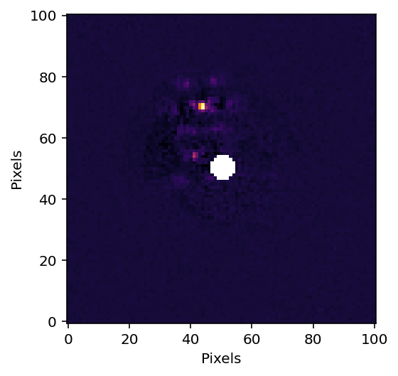
Now run pyKLIP ADI+RDI

The process here is very similar to the previous two. Because we’ll be using RDI, we’ll generate the PSF library again.

psflib.prepare_library(dataset)

parallelized.klip_dataset(dataset, outputdir="./", fileprefix=f"pyklip-{filtername}-ADI+RDI-k50a9s4", annuli=9,
                          subsections=4, numbasis=[1,5,10,20,50], mode="ADI+RDI", psf_library=psflib)


with fits.open(f"pyklip-{filtername}-ADI+RDI-k50a9s4-KLmodes-all.fits") as hdulist:
    ardi_cube = hdulist[0].data
    hdulist.close()

plt.figure()
# plot the KL20 Cube (index of 3)
plt.imshow(ardi_cube[3], interpolation='nearest', cmap='inferno')
plt.gca().invert_yaxis()
plt.ylabel('Pixels')
plt.xlabel('Pixels')

Begin align and scale images for each wavelength
Wavelength 1.0 with index 0 has finished align and scale. Queuing for KLIP
Total number of tasks for KLIP processing is 36
27.78% done (9/36 completed)
55.56% done (19/36 completed)
83.33% done (29/36 completed)
Closing threadpool
Derotating Images...
Writing Images to directory /Users/jeaadams/JWST-ERS-Pipeline/notebooks
wavelength collapsing reduced data of shape (b, N, wv, y, x):(5, 12, 1, 101, 101)

Text(0.5, 0, 'Pixels')

# Comparison plot
minval = np.nanpercentile(adi_cube[2], 0.01)
maxval = np.nanpercentile(adi_cube[2], 99.99)

fig = plt.figure(figsize=(9,5))
ax = fig.add_subplot(1,3,1)
ax.imshow(adi_cube[2], interpolation='nearest', cmap='inferno', vmin=minval, vmax=maxval)
ax.set_xlim([20,80])
ax.set_ylim([20,80])
ax.set_title("ADI", fontsize=14)
ax.set_xlabel("Pixels", fontsize=14)
ax.set_ylabel("Pixels", fontsize=14)

ax = fig.add_subplot(1,3,2)
ax.imshow(rdi_cube[2], interpolation='nearest', cmap='inferno', vmin=minval, vmax=maxval)
ax.set_xlim([20,80])
ax.set_ylim([20,80])
ax.set_title("RDI", fontsize=14)
ax.set_xlabel("Pixels", fontsize=14)
ax.set_ylabel("Pixels", fontsize=14)

ax = fig.add_subplot(1,3,3)
ax.imshow(ardi_cube[2], interpolation='nearest', cmap='inferno', vmin=minval, vmax=maxval)
ax.set_xlim([20,80])
ax.set_ylim([20,80])
ax.set_title("ADI+RDI", fontsize=14)
ax.set_xlabel("Pixels", fontsize=14)
ax.set_ylabel("Pixels", fontsize=14)
plt.tight_layout()

plt.savefig('pykip_general.png', dpic = 500)